Key Takeaways

• Modeling a Portfolio
• Modeling with Alternative Betas
• Modeling with Risk Premia
• The Intuition Behind Principal Component Analysis

Summary

Risk has long been considered an important part of portfolio construction but there have been few practical approaches to help portfolio managers assess and understand the myriad risks contained in their investment portfolios. This paper provides an overview of a risk “decomposition” approach that has been found to be applicable to a wide variety of institutional portfolios. Two methods for modeling a portfolio under this approach are presented, one using alternative betas and the other using risk premia. The results from the decomposition approach make it possible for a manager to step back and examine the overall portfolio “forest” instead of the specific investment “trees.” Further, certain applications of the technique can provide a more intuitive overview of the risk contained in a portfolio.

Introduction

The Janus Henderson Liquid Alternatives Group has developed innovative ways to measure risk in certain investments more precisely than is possible using conventional approaches. This white paper provides an overview of the theoretical basis behind the team’s approach, and is for the benefit of portfolio managers who may be interested in a richer understanding of portfolio risk.

We start from the premise that portfolio managers are rewarded for successfully investing in risk. Even when portfolio strategies are couched in terms of assets selected for investment, or returns generated by those assets, what makes the portfolio profitable is the successful selection of risk in the portfolio.

It is, of course, generally accepted that greater diversity in an investment portfolio helps to diminish the risk in the portfolio. Thus, in recent years, as portfolios have come under stress, investment managers have intensified their efforts to find and include more diversified sources of investment return. Most commonly this search has resulted in the inclusion of more and more different “asset classes” – hedge funds, real estate, private equity and the like – in portfolios. Unfortunately, these attempts at diversification are often unsuccessful; they may also introduce unnecessary and inappropriate risks into the portfolio.

It is the premise of this paper that the use of asset classes as a primary tool to determine investment choices may not paint a full picture of the underlying risks, because the same risk may be embedded in many different asset classes. We suggest that portfolio managers may gain a richer and more precise understanding of the risk inherent in a portfolio by “deconstructing” the portfolio.

Modeling a Portfolio

Scholarship in the finance industry has yielded four primary ways to model the returns of a portfolio. The first is a completely statistical decomposition, which can be done either through the use of principal component analysis (PCA) or through a technique known as statistical factor analysis (FA). The difference between the two techniques is that PCA makes no assumptions about the underlying statistical properties of the data, while FA assumes that the data are multivariate normal.¹ Statistical decomposition depends only on the return data itself to infer the factors through analysis of the variance-covariance (or correlation) matrix. Because the resulting decomposition is completely statistical, the resulting factors are not uniquely identified and are therefore generally difficult for a manager to interpret. For this reason, although PCA can help determine the extent of diversification within a portfolio by determining the number of unique risk factors, we do not recommend the use of purely statistical decomposition techniques to decompose portfolio risk since neither FA nor PCA provides a means for identification of those factors.

The second and most commonly known method for decomposing a portfolio is the use of pre-specified factors. Again, two approaches are used (although sometimes they may be combined). One uses observable equity factors such as industry classification, price to book, free cash flow and market capitalization [see, e.g., Barra (1998)]. The other uses exogenous macroeconomic factors like GDP growth, inflation, and industrial production [see, e.g., Chen, Roll, and Ross (1986)]. The use of pre-specified factors, while widespread in the industry for the construction of portfolios, often fails to capture the dynamic trading nature of an actively managed portfolio and thereby misses some of the most important portfolio risks.²

The third method, a generalization of the pre-specified factor approach, attempts to better capture dynamic risks by adding trading strategies (usually options or options-like strategies) to the fundamental and market-based factors [see, e.g,. Fung and Hsieh (1997)]. This paper refers to this method as the alternative beta approach. Finally, the fourth approach for modeling the portfolio returns uses specially constructed portfolios intended to capture fundamental risks in the market – we refer to this method as the risk premia approach. The basic idea that allows for factor decomposition is illustrated at a high level in Exhibit 1. It is our experience that these latter two modeling approaches capture, in sufficient detail, the range of risks contained in most portfolios. For that reason, we will use these last two methods to demonstrate the ideas behind our approach to portfolio risk decomposition.

Exhibit 1: The Basic Idea Behind Factor Portfolio Modeling

Exhibit 2 represents a hypothetical $100 investment in an actual, fundamentally managed $5 billion endowment from April 1995 to October 2012, with dividends and capital gains reinvested (the “value” of the endowment). The endowment’s holdings included direct investments in equity (developed and emerging markets), fixed income (sovereign and corporate), real estate (through REITs), commodities (futures) and hedge funds (direct). On a limited basis, the endowment has, from time to time, used derivatives to hedge its exposures to segments of the market. Over the period in this sample, the mean annual return for the endowment was 8.41%, the annual volatility (standard deviation of returns) was 10.22%, and the maximum drawdown experienced was -36.69%. While the endowment experienced a significant decline during the financial crisis, it recovered nicely and, from the beginning of the sample, grew almost fourfold. For the remainder of this paper, we will use this example endowment for analysis.

Exhibit 2: Endowment Performance

Hypothetical Growth of $100 (Apr. 1995 – Oct. 2012)

This hypothetical example is used for illustrative purposes only and does not represent the returns of any particular investment.

Modeling with Alternative Betas

For the first approach to modeling the returns of the endowment, we selected a set of market indices and dynamic trading strategies (alternative betas) as potential explanatory factors. The primary criteria utilized to select these indices and alternative betas were that they had to be readily priced and able to be traded in the market (albeit that some of the factors require active management). There are, therefore, no macroeconomic factors or “sentiment” factors included in the analysis.

Starting with 54 potential factors,³ we used a proprietary algorithm to select those factors that were highly cointegrated with the value of the endowment. In order to test the usefulness of the factor fit, we truncated the data set, finding those factors that provided the best statistical fit of the endowment’s portfolio for the truncated period (referred to as in-sample) with no “look ahead” bias, and then tested to see how well those factors fit the data in the ensuing months (referred to as out-of-sample). In particular, we used the period April 1995 to September 2007 as the modeling or in-sample period and the period October 2007 to October 2012 as the out-of-sample period.

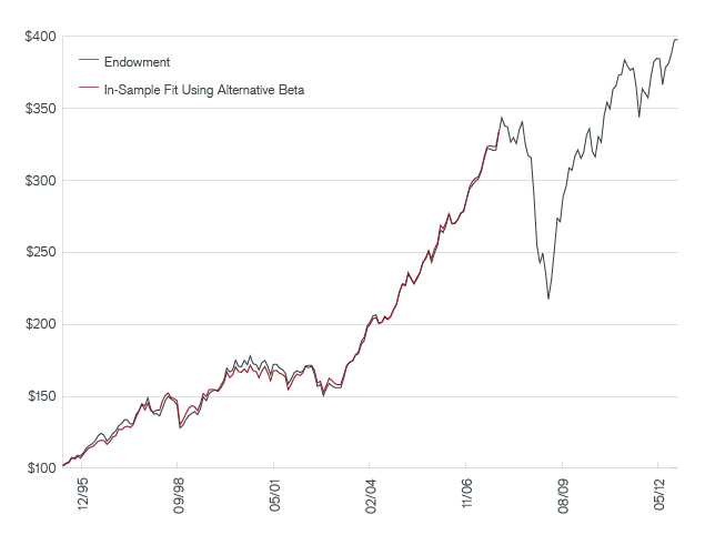
Exhibit 3 overlays the in-sample alternative beta fit (in red) on the value of the endowment (in gray). For the period April 1995 to September 2007, the endowment had a mean annual return of 10.02%, a volatility of 8.38% and a maximum drawdown of -15.48%. For the same period, the alternative beta fit had a mean return of 10.02%, a volatility of 8.07%, and a maximum drawdown of -14.36%. The correlation between the alternative beta fit and the value of the endowment for this period is 99.89.

Exhibit 3: Endowment with Fitted Alternative Beta Factors In-Sample

Hypothetical Growth of $100 (Apr. 1995 – Oct. 2012)

See below for important information regarding hypothetical and simulated performance.

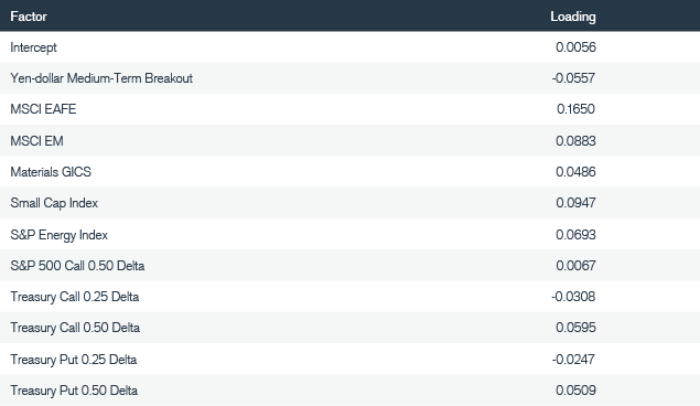
The alternative beta factors and their associated factor loadings utilized in this model (for monthly returns) are shown in Exhibit 4. Several indices are used in the model; more interesting, a number of options strategies and a yen-dollar breakout strategy are also contained in the model, which reflect dynamic risks.

Exhibit 4: Alternative Beta Model Factors and Loadings

The true test of the model is, of course, its out-of-sample performance. To evaluate this, we fix the estimated loadings on each of the factors at their values from the estimation (in-sample) period. We then use those fixed loadings and the realized returns for the factors for the October 2007 through October 2012 time period. It is important to note that this is not a forecast – we are not attempting to forecast the returns of the endowment – we are only testing whether the model remains a close approximation to the endowment’s value when taking the fixed factor loadings estimated in the earlier time period and applying them to the later period. This is a diagnostic technique for ensuring the accuracy of the model through time.

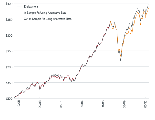
Exhibit 5 adds the out-of-sample fit (in orange) of the alternative beta model to the endowment’s value (in gray) and the in-sample model fit (in red). Considering now the entire sample period (April 1995 to October 2012), the endowment had a mean annual return of 8.41%, annual volatility of 10.22% and a maximum drawdown of -36.69%, while the combined in-sample and out-of-sample alternative beta model had a mean annual return of 8.12%, annual volatility of 9.54% and a maximum drawdown of -32.40%. The correlation between the out-of-sample alternative beta fit and the endowment for the out-of-sample period is 99.05.⁴ While we do not know the specific investments comprising the endowment, this model appears to describe the endowment quite well.

Exhibit 5: Endowment with Fitted Alternative Beta Factors In- and Out-of-Sample

Hypothetical Growth of $100 (Apr. 1995 – Oct. 2012)

See below for important information regarding hypothetical and simulated performance.

Now that we have a representative model of the endowment, we can use that model to further explore its return characteristics. We have data on the alternative beta factors dating back to January 1991, more than four years before data for the endowment became available. This data, combined with the estimated factor loadings, allows us to extend the model back in time to the beginning of 1991. We can then use the extended model to perform a Monte Carlo simulation on the returns for the model, which represents a proxy for performance over multiple sample paths in contrast with the single, actual sample path observed for the endowment. There are three steps in the Monte Carlo simulation: (1) weight the monthly return for each of the factors by the estimated factor loadings; (2) fit a t-copula to those weighted returns; and (3) draw a random sample from the fitted t-copula.⁵

Exhibit 6 represents the probability density function for annual returns as a result of the Monte Carlo simulation with 10,000 draws from the t-copula. The right-hand tail of the distribution (“good” return outcomes) is longer than the left-hand tail (“bad” return outcomes), but the distribution appears to have more mass left of zero (meaning a higher probability of bad outcomes). Indeed, the mean of the Monte Carlo simulated distribution is -0.84%, significantly different from the mean return of the endowment.⁶ Further, again in contrast with the results of the single time series of returns of the endowment, the Monte Carlo simulation for the 1991 to 2012 time period had an annual volatility of 19.99% – significantly larger than the endowment.⁷ Importantly, the maximum drawdown in the Monte Carlo simulation was -36.26%, contrasted with the maximum drawdown for the endowment of -36.69% for the entire period (April 1995 to October 2012).

Exhibit 6: Probability Density Function of Monthly Returns from Monte Carlo Simulation

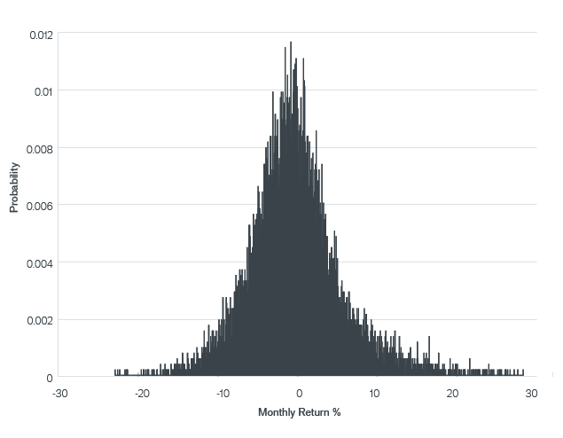
Monte Carlo Simulation is performed with a fitted t-copula using the fitted factor loadings for the period January 1991 to October 2012 – 10,000 draws. See below for important information regarding hypothetical and simulated performance.

It is important to understand what this is telling us about the returns of the endowment. We started with a model that closely fit the endowment’s value. That model was then extended back in time to generate a longer historical simulation. From that we generated a Monte Carlo simulation which provides examples of more possible outcomes that could have been realized. The Monte Carlo simulation represents 10,000 simulated monthly returns or more than 800 years of hypothetical data, as compared with the 149 months of the endowment’s data.⁸ If the model is representative of the endowment, this reveals much more information about its return characteristics. Unless, by chance, the single sample path – the endowment performance – is completely representative of the distribution of sample paths that could have been experienced, we should expect the Monte Carlo simulation to produce, on average, different results. Indeed, in this case, we can see that the distribution of possible returns was more volatile, with lower expected returns, than the endowment’s results.

This brings us to another useful piece of information that can be extracted from the Monte Carlo simulation: loss probabilities. Exhibit 7 gives the potential one-month loss associated with various probabilities. From the Monte Carlo analysis, we can determine that the probability of losing more than 12% in a month was 1%.

Exhibit 7: Monte Carlo Estimated Loss Probabilities (one month)

Monte Carlo Simulation is performed with a fitted t-copula using the fitted factor loadings for the period January 1991 to October 2012 – 10,000 draws. See below for important information regarding hypothetical and simulated performance.

Modeling with Risk Premia

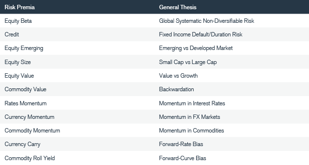
While we could continue to use this existing model for further analysis, it is our view that a different approach to the alternative beta approach – the use of risk premia – provides a more complete understanding. Risk premia can be thought of as the total (or absolute) return associated with investing in – or the assumption of – a specific type of risk in the market. The best-known risk premium is systematic equity risk – the general market risk, or non-diversifiable risk, associated with an otherwise well-diversified portfolio of equities. This is the risk upon which the foundation of Modern Portfolio Theory was laid [see, e.g., Markowitz (1952) and Sharpe (1964)]. Over time, however, additional risk premia have been discovered and documented [see, e.g., Fama and French (1993); Banz (1981); Chan, Jegadeesh, and Lakonishok (1996); and Chan, Karceski, and Lakonishok (1998)]. Exhibit 8 lists the risk premia used in this study and the general underlying thesis associated with each. Note that while risk premia represent expected compensation for certain risks, as stated in the name “risk premia” there is inherent risk associated with each and no guarantee of returns.

Exhibit 8: Risk Premia

The use of risk premia to model the returns of the endowment follows the approach used previously for alternative betas. In this case, however, we do not have as long a time series of risk premia, so the modeling covers the period from January 2000 to October 2012.⁹ Following the framework presented earlier, Exhibit 9 plots the endowment’s value (now starting in January 2000) in gray, the risk premia model in-sample (January 2000 to September 2007) fit in red and the risk premia model out-of-sample (October 2007 to October 2012) fit in orange. The in-sample fit has a correlation of 99.81 with the endowment’s value and the out-of-sample fit has a correlation of 99.14 with the endowment’s value.

Exhibit 9: Endowment with Fitted Risk Premia In- and Out-of-Sample

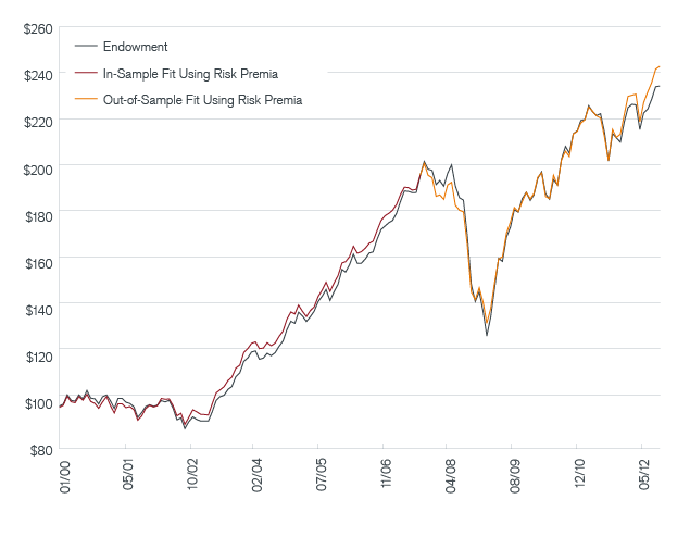
See below for important information regarding hypothetical and simulated performance.

Exhibit 10 presents the summary statistics for the risk premia model and the endowment.

Exhibit 10: Endowment and Risk Premia Model Summary Statistics

Although we used a shorter time series to fit the risk premia model to the endowment’s data, this model also appears to fit the data quite well. Exhibit 11 details the risk premia and their associated factor loadings in this model. Note that fewer risk premia are needed in this model than factors in the alternative beta model; moreover, the risk premia may have broader intuitive appeal than the alternative betas as they represent broad trading strategies rather than investments in specific securities. Now, using the risk premia model we can address another important issue for a fund manager: measuring the degree of diversification in the portfolio.

Exhibit 11: Risk Premia Model Factors and Loadings

The basic concept of diversification is simple: “don’t put all of your eggs in one basket.” The hope is that if a portfolio holds a variety of instruments (that are not perfectly correlated with each other), when some investments go down, others will go up, such that the portfolio will be better off than it would have been without diversification. The problem facing a manager is that there is no commonly accepted measure of diversification, although many have been proposed. There are measures based on the tradeoff between risk and return [see, e.g., the Sharpe Ratio (1964); the Treynor Measure (1965); and Jensen’s Alpha (1968)]. Each of these measures combines the expected benefit of diversification – risk reduction – with the objective of the investment process – return. Using this approach as a measure of diversification confuses the issue, instead of directly addressing the question of how many different risk exposures are represented in the portfolio. Other measures attempt to directly answer the question of diversification – e.g., the Herfindahl Index (1955) (a measure of economic concentration based on the size of the holdings in the portfolio); the Rosenbluth Index (1961) (based on rank ordering of the size of the holdings in the portfolio); and the entropy measure by Hart (1971) (based on weighted average of the size of the holdings in the portfolio).¹⁰ These measures, however, all suffer from the underlying assumption that the portfolio holdings are all uncorrelated with each other – an assumption that is clearly not justified.

A theoretically more straightforward approach to measuring the diversification in a portfolio is to decompose the risk of the portfolio into a set of independent components.¹¹ Then, simply by counting the number of independent components that capture a specific amount of the risk, we have a measure for the degree of diversification in our portfolio. A standard statistical technique for this type of decomposition is principal component analysis or PCA¹² (see below for an explanation of PCA).

The Intuition Behind Principal Component Analysis*

In any complex system, like the financial markets, much of the data we receive is a noisy signal of the true, underlying data. For example, we cannot directly observe the inflation-adjusted interest rate – instead, we (or others) estimate that rate based on both an estimate of inflation and an estimate of the interest rate reflected in bonds that trade relatively infrequently. Similarly, what is the price of any given stock today? Is it the closing price, the opening price, the volume weighted average price (VWAP), or the average of the high and low for the day? Moreover, the information in equities has something to say about inflationary expectations, and the information in interest rates provides information about expected returns in equities. When we consider all investments in a portfolio, this redundancy becomes even more apparent – different bond returns contain much of the same information, as do different equity returns. All of this data can, at times, appear to be much more complex than it is. In fact, typically only a few drivers account for the majority of the variation in the data. Principal Component Analysis provides a statistical method for reducing a complex data set to a simpler one.

Imagine a ball suspended from a spring attached to the ceiling.** One way to study the motion of the ball would be to arrange around the room a series of cameras that could photograph the ball as it bounced on the spring. While we could use hundreds of cameras, the location of a camera that would capture the majority of the motion of the ball would be a camera directly perpendicular to the ball and spring. That camera would represent the first principal component of the motion of the ball. Note that this camera is not unique, since any other camera located in a circle perpendicular to the up and down movement of the ball would work just as well. If we wanted to isolate any back and forth “jiggle” in the path of the ball, we might place a camera directly below the ball looking up – that would represent the second principal component.

In this example, the first principal component would capture the majority of the motion of the ball. In fact, PCA generally ranks the principal components in order from the largest (which explains most of the variation) to the smallest (which explains the least amount of the variation). The principal components are constructed to be independent and uncorrelated with each other and to explain all variation in the data. The primary failing of PCA is that the principal components cannot be uniquely identified – remember that the first camera could be placed anywhere on the circle perpendicular to the ball and spring. While this limits the usefulness of PCA for identification of the risks in a portfolio, it does not diminish its usefulness for determining the degree of diversification.

* The technical details of PCA can be found in standard statistical texts – see, e.g., Chatfield and Collins (1980).
** This is abstracted from Shlens (2009).

Exhibit 12, which indicates the results of a PCA decomposition for the modeled endowment, is striking. The first principal component accounts for 94.97% of the variance in the modeled portfolio. This fact, combined with the relative size of the remaining principal components in the modeled portfolio, indicates that the endowment which the model was based on was not particularly well diversified.

Exhibit 12: PCA Decomposition of Risk Premia Modeled Portfolio Allocation

Percent of Variance Explained (Jan. 2000 – Oct. 2012)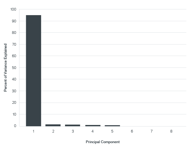

This analysis is based on a hypothetical modeled portfolio and is used for illustrative purposes only.

The risk decomposition modeling approach can also be used for attribution of returns. In the case of the risk premia model, return attribution can be directly interpreted as answering the question: How much is the investor being compensated for the specific risks taken in the portfolio? Using the risk premia model and its associated loadings, Exhibit 13 shows the percentage of total return contributed from each of the risk premia for the model portfolio over the one-year period from November 2011 to October 2012. Similarly, Exhibit 14 shows the same results for the five-year period from November 2007 to October 2012.

Exhibit 13: Contribution to Total Return: Risk Premia Model

Contribution from Risk Premia (Nov. 2011 – Oct. 2012)

See below for important information regarding hypothetical and simulated performance.

From Exhibit 13, it is apparent that the risk associated with commodity roll yield (a short position, as indicated by the loadings) did not, in aggregate, add to the return of the endowment, but that positions in the other risk premia contributed significantly to its simulated performance during the one-year period. The dominant contributors to the simulated performance over the five-year period were equity beta, equity size and credit. However, as starkly illustrated in Exhibit 14, the exposure associated with commodity roll yield produced a significant drag on simulated performance over the five years.

Exhibit 14: Contribution to Total Return: Risk Premia Model

Contribution from Risk Premia (Nov. 2007 – Oct. 2012)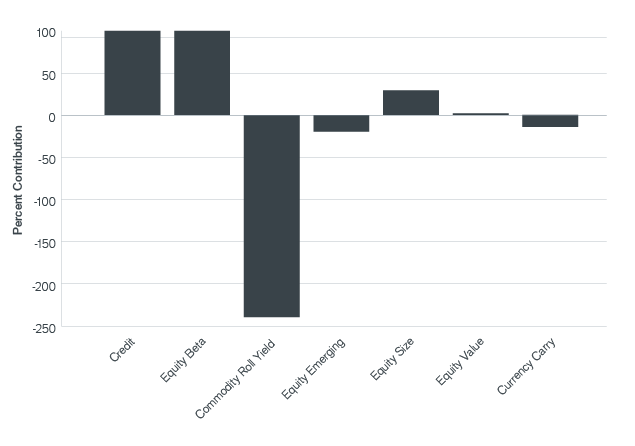

See below for important information regarding hypothetical and simulated performance.

Exhibit 15 represents a hypothetical $100 invested in each of the model risk premia over the 12-year period (weighted by the model loadings). This highlights the relative performance of each risk premia over time for the simulated portfolio. As we might expect, equity beta, equity emerging and credit all contributed to simulated performance (and it is apparent that equity beta provided significant volatility); the other equity-based risk premia and currency carry had lackluster performance, and the position in commodity roll yield was a drag on performance for the entire period.

Exhibit 15: Model Risk Premia

Hypothetical Growth of $100 (Jan. 2000 – Oct. 2012)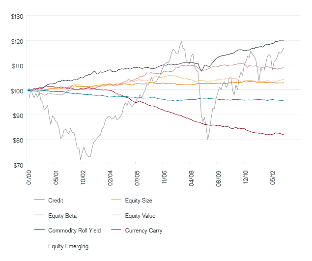

See below for important information regarding hypothetical and simulated performance.

Conclusion

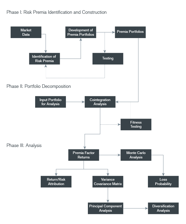
In this paper, we have presented an approach to modeling a portfolio that we believe facilitates better understanding of its risks, which makes it possible to “step back” and examine the overall portfolio “forest” instead of the specific investment “trees.” Two methods for modeling a portfolio were presented, but they both rely on the same underlying approach – factor decomposition of the portfolio. Exhibit 16 details the logic flow used for risk premia modeling, but the same logic can be applied to modeling with alternative betas. Each modeling method has its pluses and minuses: alternative betas can be constructed with longer histories and can be directly traded in the market. But, it can be difficult to develop good intuition about some of the dynamic factors and some of the alternative betas may not be stable through time. Risk premia tend to provide a more parsimonious description of the portfolio and, at least in the broad sense, are more intuitive. However, it is technically more difficult to construct the underlying portfolios that constitute the risk premia.

By focusing on the risks of the portfolio – not the risks associated with specific investments or particular asset classes – managers can begin to make better decisions about their portfolios. It is our hope that the approach detailed in this paper will help to make that possible.

Exhibit 16: Risk Premia Modeling Process

References

Banz, R., “The Relationship Between Return and the Market Value of Common Stocks”, Journal of Financial Economics, 1981, 9, 3-18.

Barra, “Single Country Equity Risk Model”, 1998.

Chan, L., N. Jegadeesh, and J. Lakonishok, “Momentum Strategies”, Journal of Finance, 1996, 51:2, 1681-1713.

Chan, L., J. Karceski, and J. Lakonishok, “The Risk and Return from Factors”, Journal of Finance and Quantitative Analysis, 1998, 33:2, 159-188.

Chatfield, C. and A. Collins, Introduction to Multivariate Analysis, Chapman and Hall, London, 1980.

Chen, N., R. Roll, and S. Ross, “Economic Forces and the Stock Market”, Journal of Business, 1986.

Fama, E. and K. French, “Common Risk Factors in the Returns of Stocks and Bonds”, Journal of Financial Economics, 1993, 33, 3-56.

Fung, W. and D. Hsieh, “Empirical Characteristics of Dynamic Trading Strategies: The Case of Hedge Funds”, The Review of Financial Studies, Summer 1997, 10:2, 275-302.

Hart, P., “Entropy and Other Measures of Concentration”, Journal of the Royal Statistical Society, 1971, 134, 73-85.

Henriksson, R. and R. Merton, “On Market Timing and Investment Performance II. Statistical Procedures for Evaluating Forecasting Skills”, Journal of Business, 1981, 54, 513-533.

Herfindahl, O., “Comment on Rosenbluth’s measures of concentration” in Stigler, G. (ed.), Business Concentration and Price Policy, 1955, Princeton University Press.

Jensen, M., “The Performance of Mutual Funds in the Period 1945-1964,” Journal of Finance, May 1968, 23:2, 389-416.

Markowitz, H., “Portfolio Selection”, Journal of Finance, 1952, 7:1, 77-91.

Mergenthaler, K. and H. Zhang, “Public Pension Funds: Asset Allocation Strategies”, JP Morgan Investment Analytics & Consulting, www.jpmorgan.com, 2010.

Merton, R., “On Market Timing and Investment Performance I. An Equilibrium Theory of Value for Market Forecasts”, Journal of Business, 1981, 54, 363-406.

Nesbitt, S., “Trends in State Pension Asset Allocation and Performance”, www.cliffwater.com, 2012.

Rosenbluth, G., “Address to Round-Table-‘Gesprach uber Messung der industriellen Konzentration'”, in Neumark, F. (ed.), UI, in Schriften des Vereins fur Socialpolitik, 1961, N.S., 22, 391-394.

Rubinstein, M. and H. Leland, “Replicating Positions in Options with Stocks and Cash”, Financial Analysts Journal, 1981, 37, 63-75.

Sharpe, W., “Capital Asset Prices: A Theory of Market Equilibrium under Conditions of Risk”, Journal of Finance, 1964, 19:3, 425-442.

Shlens, J., “A Tutorial on Principal Component Analysis”, Working Paper, April 2009.

Towers Watson, “Global Pension Assets Study 2012”, www.towerswatson.com

Treynor, J., “How to Rate Management Investment Funds,” Harvard Business Review, January-February 1965, 43:1, 63-75.

Woerheide, W. and D. Persson, “An Index of Portfolio Diversification”, Financial Services Review, 1993, 2(2), 73-85.

---

1. The technical details associated with both of these techniques can be found in any standard text on multivariate analysis, see, e.g., Chatfield and Collins (1980).
2. Market timing skill and dynamic trading strategies introduce option-like characteristics to a portfolio [for market timing skill see, e.g,. Merton (1981), and Henriksson and Merton (1981); and for dynamic trading strategies see, e.g., Rubinstein and Leland (1981)].
3. Generically, these are broad indices representing equities, commodities and fixed income (covering both developed and emerging markets), trading strategies in those indices and futures (including foreign exchange) which capture trends and breakouts, and option strategies that capture volatility trading strategies in the same universe of assets.
4. Note that this out-of-sample fit is for a period of almost five years without an updating of the factor loadings.
5. The technical details are beyond the scope of this paper. A t-copula is used because it allows for the existence of “fat-tails” in the return distribution.
6. Recall that the endowment had an annual mean return from April 1995 to October 2012 of 8.41%.
7. The endowment had an annual volatility from April 1995 to October 2012 of 10.22%.
8. For the computation of maximum drawdown, this only represents 47 sample paths of the time period April 1995 to October 2012, but we have also run Monte Carlo simulations with 100,000 and 1,000,000 draws or 500 and 5,000 sample paths respectively – the means, volatilities and maximum drawdowns are all consistent with the results presented here.
9. Construction of a longer time series of these specific risk premia portfolios is not possible because of structural changes in the market, for instance the advent of the euro.
10. For a more complete discussion and analysis of these types of portfolio diversification measures, see Woerheide and Persson (1993).
11. The factors identified in the modeling discussed above are not, in general, independent in the statistical sense – there is a correlation structure inherent in the factors.
12. More technically, PCA decomposes the volatility into linearly independent, uncorrelated and orthogonal components.