Key Takeaways

• Assessment of how terminal portfolio value is impacted much more by a few large moves, both positive and negative, than many small moves.
• Overview of the drag that time-varying risk and tail risk have on long-term portfolio value.
• Analysis of how diversifying risk across time can reduce this drag.
• Benefits of an investment approach focused on outliers and away from averages to maximize terminal portfolio value.

Introduction

Though most investors may not be explicit in saying it, one of their primary goals is increasing the “terminal value” of their investments – i.e., maximizing the growth of an investment over time – for a desired level of risk. Pensions focus on long-term assets relative to liabilities, endowments and foundations on compound returns relative to spending rates, individuals on saving enough for future retirement needs. Yet, professional investors manage portfolios with a goal of maximizing per-period averages per unit of average risk, like Sharpe or information ratios. This raises the question: Is the goal of maximizing measures like Sharpe ratio or information ratio consistent with the goal of maximizing terminal value? The answer is a resounding no.

Managing portfolios to enhance averages – like Sharpe or information ratios – is a very different goal compared to that of enhancing terminal value. The optimality of maximizing Sharpe or information ratios is rooted under the assumption of repeatable single-period investing, while enhancing terminal value is rooted in multi-period investing, where the environment from one period to the next can be very different. The risk of a portfolio over a single period is managed by diversifying holdings – cross-sectional diversification. But once time enters the picture through an emphasis on terminal value, diversifying across time becomes even more important than diversifying across assets. This time diversification is crucial because the level of asset class risk fluctuates, sometimes violently, across time, leading to a form of convexity costs. Most know that convexity costs arise from noise (volatility) around realized returns and result in a drag on compound returns. But what is less known is the fluctuation in risk levels over time, which we call excess risk, amplifies these costs.

While there is little one can do to remove the noise around realized returns to reduce convexity costs, excess portfolio risk can be addressed with time diversification. Diversifying across time reduces the drag on compound returns by decreasing the fluctuation in risk levels to maintain a constant risk level from period to period – a target risk level. The “convexity cost” of this excess risk can be large – resulting in a meaningful reduction in compound return. This is true even if asset returns follow a normal distribution. Portfolio management should seek to reduce this cost by reducing the fluctuations in risk around target levels.

In practice, convexity cost can be greater than many expect as asset return distributions are fat-tailed and the large negative outliers lead to a much larger drag on compound returns than volatility moves. Therefore, portfolio management should develop measures of risk consistent with this reality: tail risk is the most important risk affecting compound returns. The impact on terminal value of just a few outliers, both positive and negative, is much greater than that of many small moves.

We propose an investment approach – which we call adaptive asset allocation – that refocuses the goal of portfolio management toward maximizing terminal value. In this approach, portfolios adapt to current market conditions with an eye toward both the present (cross-sectional diversification) and the future (time diversification).

Interestingly enough, static averages and conventional measures of portfolio efficiency can mask the opportunity presented by adaptive asset allocation: both the information ratio and Sharpe ratio¹ may show little advantage to the approach, at least at times. Yet, the positive impact on terminal value can be substantial.

Beginning with the assumption that the goal is to maximize terminal value for a given target risk level, this paper outlines two key concepts that drive terminal value: time diversification and convexity costs, specifically the amplification of these costs due to fat tails. We conclude with a high-level overview of adaptive asset allocation, an investment approach that seeks to enhance terminal value by dynamically managing portfolio outliers.

Time Diversification: A New Dimension in Risk Management

Managing portfolios to maximize terminal value adds a new dimension of risk: time. Terminal value is a reflection of portfolio value growth over multiple periods as returns compound. As a result, risk must be managed across more than just a single period. The impact of risk over time is ignored in most investment models, which focus on a single period. In a single-period model, the only risk that can be managed is cross-sectional risk through holding a diversified portfolio of assets. However, once time enters the picture, risk can also be diversified across time – and the impact of diversifying across time can be much greater than diversifying in the cross section.

To illustrate, consider an investor with $100 million of capital. For 99 days, the investor risks $1 million in a portfolio diversified across multiple assets. Then, on the 100th day, the investor risks all $100 million in the same portfolio. This portfolio is “diversified” in the sense that it has balanced risk across a number of assets in each single period. However, it has failed to balance risk across time. The potential for a 100% loss on the final day results in far greater risk to terminal value than all of the previous days combined.

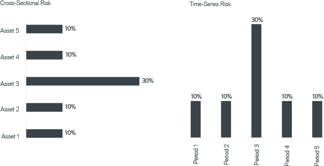
This idea is highlighted with a more realistic example in Exhibit 1, which shows the risk of hypothetical assets at one point in time on the left and the risk of a portfolio across time on the right. Just as a cross-sectionally diversified portfolio would reduce the relative weight to the riskier Asset 3, so too would a time-diversified portfolio reduce the relative weight to the riskier Time Period 3. Both forms of diversification will reduce the risk around the average, the former across one period and the latter across multiple periods.

Exhibit 1: Cross-Sectional vs. Time-Series Risk

Assessing Risk Across Assets and Time

Ignoring changes in risk over time can have serious consequences for terminal portfolio values. Even so-called “balanced” portfolios can have dramatically varying risk over time. As an example, rolling standard deviations of a 60/40 portfolio are shown in Exhibit 2. At times, the risk of the strategy is high. At other times, it is low. The highly variable risk of the “balanced” portfolio over time results in a lack of time diversification.²

Exhibit 2: Annualized Rolling Three-Year Standard Deviation of 60/40 Portfolio

The Impact of Time-Varying Risk

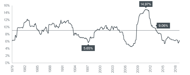
Source: Bloomberg. 60/40 MSCI World Index/Bloomberg Barclays U.S. Aggregate Bond Index. As of 12/31/2018.

Current portfolio construction approaches determine allocations without taking account of varying expected risks over time. The result is often wildly changing levels of portfolio risk, which can create a significant drag on performance – and one that is not captured in per-period means and variances. Consider the following simple examples:

• Average performance is realized over identical and repeatable periods: Imagine a coin showing heads half the time and tails half the time. With just four flips, it is not so likely that half the flips will be heads. But with 1,000 flips, it is very likely that close to half will be heads. That is the power of repeating the game and repeating the same scenario: you realize the average outcome.
• Averages ignore the effects of compounding across non-identical periods: Investors do not have the luxury of living in a single-period, repeatable world – or a world of averages. An investment that gains 50% today and loses 50% tomorrow has an average return equal to zero. But this is not the case in a multi-period compounding world where capital put at risk varies. Gaining 50% today and losing 50% tomorrow yields an overall loss in portfolio value of 25%, very different from the “average return” of zero.

We invest not over repeatable single periods, but across non-identical multiple periods. And investing across multiple periods adds the time dimension to the risk. If one cares about terminal value, one needs to refocus attention and effort away from modeling the averages and toward reducing the variability of portfolio risk from target risk over time. Doing so can reduce portfolio return drag from excess risk, or convexity cost.

Reducing Convexity Costs Can Help Maximize Terminal Value

The time-varying level of risk in a portfolio can significantly reduce compound returns. And most investors make inaccurate assumptions about how changing risk levels can impact terminal value, if at all. Imagine two portfolios with the same expected return targeting a beta of 0.5 to the equity market:

• Portfolio A invests fully in U.S. equities 50% of the time and fully holds cash otherwise.
• Portfolio B holds 50% of U.S. equities and 50% of cash at all times.

These two portfolios both have an expected return equal to 50% of the expected market return, but will not yield the same terminal value. The risk of Portfolio A changes over time from zero (when only cash is held) to that of the risk of U.S. equities (when only U.S. equities are held). While both have a 0.5 beta, the fluctuation in risk causes the volatility of Portfolio A across time to be about 70% of U.S. equities and not one-half. And it is this excess volatility that results in convexity cost. This cost can be avoided by time diversification. Portfolio B is a time-diversified strategy whose risk stays at 50% of the risk of U.S. equities at all times and hence doesn’t suffer the convexity drag.

As shown in Exhibit 3, the drag is significant: Portfolio B compounds wealth 50 basis points (bps) per year faster than Portfolio A. Over 90 years, $1,000 invested in Portfolio A grows to $32.500, while $1,000 in Portfolio B grows to $107,200. The power of time-series diversification is that terminal value is enhanced without requiring the ability to predict expected returns. All that is required is to reduce the variability of risk around a target level. And in this case, that translates to maintaining a fixed exposure to the U.S. market versus varying exposure over time.

Exhibit 3: Comparing Equal Beta Portfolios with Time-Varying Levels of Risk

The Costs of Fluctuating Portfolio Risk Over Time

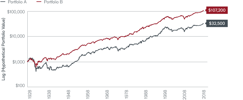
Portfolio A alternates between investing in the S&P 500 Index and holding cash (3 Month Treasury Bill) every other month, while portfolio B holds half cash and half the S&P 500 Index each and every month. For this analysis we define the return associated to U.S. equities in the S&P 500 Index as the return in excess of cash.

For those underwhelmed by this improvement, there are two key points to consider:

• Due to the effect of compounding, even modest increases in compound return lead to meaningful increases in terminal value.
• More importantly, this example uses volatility as a measure of risk to illustrate the concept of convexity costs. In practice, volatility is an inadequate measure of risk as asset return distributions are fat-tailed. The impact of outliers on terminal value is large, and their presence can drive convexity costs significantly higher

The Impact of Outliers: Convexity Costs May be Larger Than You Think

Given a focus on maximizing terminal value, it is important to diversify risk across time to reduce convexity costs that arise due to time-varying risk levels. With this goal in mind, an important question remains: what measure of risk should we diversify across time?

Due to their outsized impact on terminal value, the measure of risk should account for large tail losses and tail gains. Large positive or negative returns have a much greater impact on terminal value than many small returns. For example, losing 50% in one period requires that the portfolio accumulate a total return of 100% over subsequent periods to return to the accumulation phase again. And returning to the accumulation phase may take quite a while if portfolio risk is reduced following the drawdown. This is a common result due to portfolio investment constraints, which can call for reductions in risk levels after sustained losses. Such constraints can further increase variability of risk around target levels, and thus convexity costs.

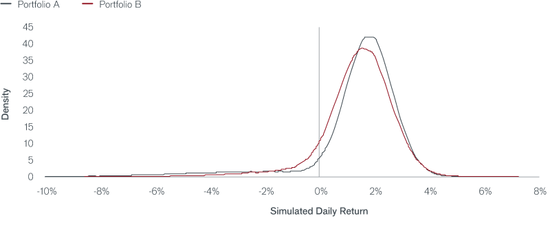
Exhibit 4 demonstrates, in a simulation setting, the asymmetric impact that a few large outliers have on compound returns. It highlights that convexity costs can be much larger in the presence of fat tails. The reason being when drawing from the fat-tailed part of a distribution, the risk is remarkably different from drawing from the non-fat-tailed part, leading to large variation in risk over time. Exhibit 4 compares the differences in compound returns between two portfolios that have identical means, but differ in their tail and “non-tail” properties – the moves between the 10th and 90th percentiles (representing 80% of all of the moves). These tail properties are shown as expected tail loss and expected tail gain. Expected tail loss (ETL) is defined as the average returns below the 10th percentile and expected tail gain (ETG) as that above the 90th percentile. In Exhibit 4:

• Portfolio A has a fat left tail and Portfolio B has a left tail one-third smaller.
• Portfolio A and B have equal right tails.
• Portfolio A has a higher average return in the non-tail region that represents 80% of days.
• Both portfolios have the exact same average annual return of 7.7%.

To summarize, Portfolio A (the fatter-tailed distribution) underperforms in the worst 10% of instances, performs at par in the 10% best cases and outperforms Portfolio B 80% of the time.³ Yet both have the same expected return. To equate the means of the two distributions, the many “non-tail” moves of Portfolio B are pulled downward. What is gained in per-period average returns from reducing the left tails equals what is lost by shifting the many small non-tail moves lower.

Exhibit 4: Convexity Costs, Outliers and Terminal Values

Fat Left Tails and the Gains from Reducing Convexity Costs

Simulated Performance	Portfolio A	Portfolio B	Difference
Compound Return	4.4%	5.6%	1.2%
Average Annual Return	7.7%	7.7%	0.0%
Volatility	24.5%	19.1%	-5.4%
Daily Expected Tail Loss (ETL)	-3.9%	-2.6%	-33.0%
Daily Expected Tail Gain (ETG)	1.9%	1.9%	0.0%
Daily “non-tail” move	0.29%	0.13%	0.16%
“Left-Tail Fatness” (ETL/ETG)	2.06	1.38	66.7%

In the framework of Exhibit 3, one can conceptually think of Portfolio A investing some of the time in an asset whose returns are normally distributed and some of the time in an asset whose returns follow a jump-down process. And one can think of Portfolio B investing all the time in an asset whose returns are nearly normally distributed, hence less fat-tailed. Intuitively, Portfolio A could represent a short volatility or long carry strategy, while Portfolio B does not.

Despite both Portfolio A and B having the same expected return, Portfolio B achieves an increase in compound return of more than 120 bps per year. The fluctuation in the risk taking of Portfolio A, which at times is exposed to normal risk and at other times is exposed to jump risk, results in a convexity cost and this time the convexity cost is much larger than in Exhibit 3 because the risk that is fluctuating is tail risk. The impact of the tail returns on terminal value is outsized relative to “non-tail” returns.

This shows that reducing convexity costs in the presence of larger left tails, rather than smaller left tails, accrues greater benefit to terminal value – even at the expense of lower average returns the majority (80%) of the time. The reverse would be true for large right tail gains. A few large moves, either positive or negative, impact terminal value far more than many small moves. Therefore, tail risk, not volatility or standard deviation, is the natural measure of risk to diversify across time when the goal is maximizing terminal value.

Toward an Adaptive Asset Allocation Approach

The adaptive asset allocation approach seeks to achieve investor goals, while accounting for the underappreciated risks highlighted in this paper. The adaptive asset allocation approach:

• Seeks to increase terminal value and manage risk
• Emphasizes time diversification in addition to cross-sectional diversification
• Reduces convexity costs with a focus on reducing tail losses and capturing tail gains

Adaptive asset allocation adapts to changing risk levels and changes portfolio weights to help avoid detrimental tail risks, i.e., suffering a tail loss or failing to participate in a tail gain. Whereas most investment approaches spend the majority of time and effort on average outcomes, adaptive asset allocation seeks to manage outcomes that have the largest impact on terminal value, namely left and right tail events.

When measured relative to a benchmark whose risk varies over time, adaptive asset allocation aims for a significant reduction in downside loss. As a result, it can create strong outperformance on the downside (alpha). At the same time, it aims to retain the majority of upside performance by additionally concentrating on right tails. Although per-period alpha may not be very large from avoiding a few very bad outcomes or participating in a few large gains, these events have a disproportionate impact on terminal value. The effects of this time diversification can be magnified in practice, as macro-shocks can result in spikes in asset class correlation resulting in fat-tailed distributions of seemingly diversified portfolios or indices.

While adaptive asset allocation adds the element of time diversification, it does not overlook cross-sectional diversification. Although macro-shocks that devastate terminal values are relatively infrequent, “micro-shocks” across sub-asset classes are more common. Steep drops in individual assets due to events such as earnings announcements or commodity price shocks occur relatively frequently. Anticipating these micro-shocks and adapting portfolio risk accordingly can reduce cross-sectional convexity costs, further enhancing terminal values.

In sum, the adaptive asset allocation approach is not a single portfolio, but rather a portfolio management mindset. Once we accept that the true goal of most investors is, in fact, maximizing terminal portfolio values for chosen risk levels, we must refocus the diversification approach toward the time dimension and the portfolio management approach toward the outliers, both of which are the factors that have the biggest impact on terminal portfolio values.

In Summary

Time diversification is ignored in most standard models in finance, which fail to account for impacts on terminal value from deviations in risks from target levels over the investment period, which we call excess risk. This excess risk significantly reduces compound returns and terminal value by magnifying convexity costs. The form of excess risk that most negatively impacts terminal value is left-tail risk. Conversely, right-tail risk results in the largest increases in terminal value.

As such, we believe that investors would benefit from adaptive asset allocation that focuses on outsized moves – reducing portfolio risk when downside tail risk increases and increasing portfolio risk when upside tail risk increases. This approach exhibits strong time-series diversification, and convexity gains, especially relative to other common asset allocation approaches. Moreover, cross-sectional diversification must not be forgotten. While the benefits of cross-sectional diversification disappear during a crisis, wherein seemingly unrelated assets exhibit high correlations, the benefits from managing micro-shocks are clear in non-crisis periods. We believe that changing the focus from relative performance measurement and benchmarking to an adaptive asset allocation approach, which takes into account the changing risks of the benchmarks and their components, will manage portfolio risks more efficiently and enhance terminal value, and do so more consistently over time.

---

1. Information ratio measures per-period average excess portfolio return over its benchmark, divided by the excess return volatility; Sharpe ratio measures per-period average return of the portfolio in excess of the riskless rate, divided by the volatility of the portfolio.
2. The risk of a cross-sectional diversified index, like the S&P 500 Index, also varies over time, leading to a lack of time-series diversification and causing those that track the index to suffer large convexity costs.
3. Based on 10,000 ten-year paths.