Subscribe
Sign up for timely perspectives delivered to your inbox.
Sustaining growth while taming inflation is the navigation challenge facing central banks. The Global Bonds Team model how different fixed income sectors could fare in various scenarios.


Welcome to the first edition of our bond market forecast analysis. This report is based on the scenario analysis run by the Global Bonds Team to guide asset allocation decisions. Each report tries to assess the expected returns potentially delivered by the major fixed income sectors based on a range of modelled outcomes (see appendix for a full description of our methodology).
After the worst start to the year in history, things can only get better. Right? But with more hawkish language from central banks and growth starting to fade, the global economy is now treading a very fine line between policy error and soft landing. The chance of policy error has grown over recent months as central bankers have had to aggressively hike rates to try and tame inflation. But have we forgotten monetary policy usually works with a lag? Although inflation has continued to beat expectations, there are now numerous indicators signalling a reduction of the supply/demand imbalance that had stoked prices since the pandemic. Freight rates are falling dramatically – with new ships and capacity all expected to step up next year – while commodity prices are in decline, and finally, the PMI and ISM surveys have started to indicate economic output is slowing around the world.
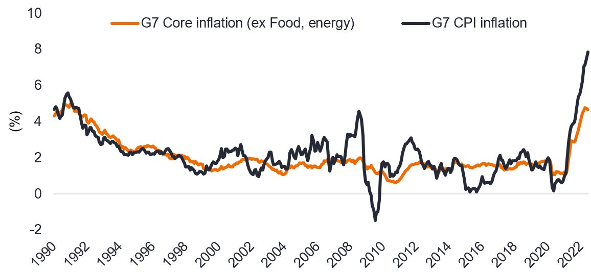
Source: Janus Henderson Investors, Bloomberg, as at 30 June 2022. Notes: OECD major seven economies CPI.
The conflict in Russia continues to cloud the economic outlook, however. Should Russia follow through on threats to cut off gas to Europe, the resulting chilling effect on growth would be felt globally.
We adopt a scenario-driven approach to identify the relative attractiveness of fixed income sectors. Our aim is not to perfectly forecast returns to the nearest basis point (as that is not possible), but to understand the range of return outcomes and gauge the resilience of that performance across probable growth scenarios.
Our base case over the next 12 months to end of June 2023 is that the global economy enters a recession largely due to the conflict in Ukraine and weakening consumer spending as real incomes are eroded by inflation, with labour market pressures moderating. In the US for example, we model core inflation peaking in September and falling to around 3.3% at the end of the period, limiting the need for additional rate hikes in 2023.
Overall, the chances of more growth lengthening this current growth cycle are looking increasing unlikely. To put this in context, we only see a one in three chance of either of our two growth scenarios materialising.
Base case (shallow recession):
Bear case (deeper recession):
Bull case (high pressure economy):
Extreme bull case (armistice):
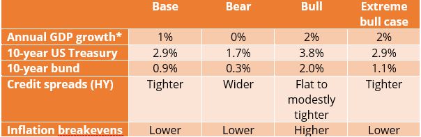
Source: Janus Henderson Investors, 21 July 2022. *Average for US/EU GDP growth over the 12-month period. There is no guarantee that past trends will continue, or forecasts will be realised.
2022 has been the worst start to any year on record for fixed income total returns. Nevertheless, rate hikes and wider credit spreads have significantly improved forward-looking returns (as shown by the positive expected returns in the base case scenario). Moreover, there is currently no single asset class that particularly stands out as being particularly mispriced. As such, we see benefits in asset diversification at this point in the economic cycle, not least given the uncertainties around economic outcomes and central bank policy.
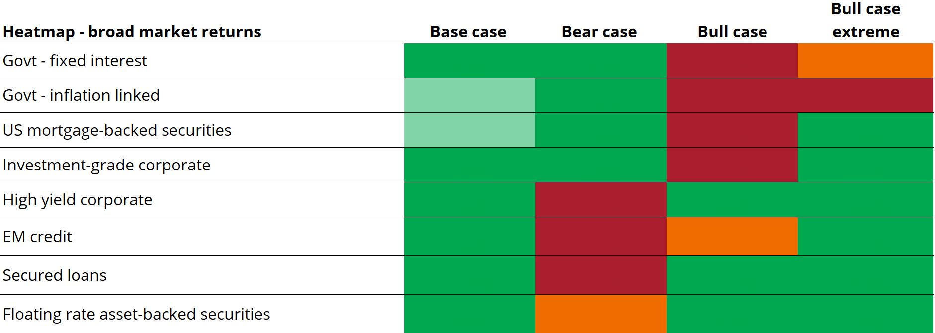
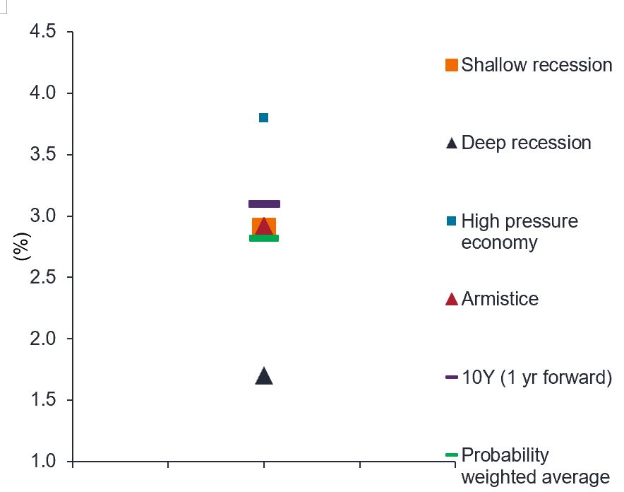
Legend: 1-year sector return estimates (%) in each scenario

Source: Janus Henderson Investors, as at 21 July 2022. Note:*Bull (bear) refers to a positive (negative) outturn for economic performance. Expected returns for a US dollar-based investor, based on index returns before allowance for alpha. Any differences among portfolio securities currencies, share class currencies, and your home currency will expose you to currency risk. The above are the portfolio managers’ views and should not be construed as advice and may not reflect other opinions in the organisation. There is no guarantee that past trends will continue, or forecasts will be realised.
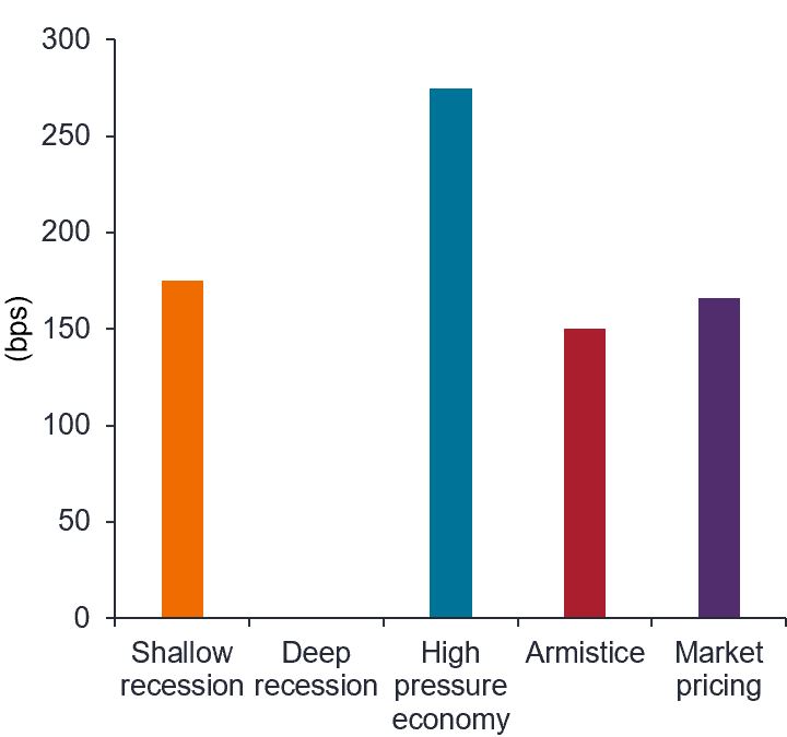
Note: no rate hikes are expected in the ‘Deep recession’ scenario.
Source: Janus Henderson Investors, 21 July 2022. There is no guarantee that past trends will continue, or forecasts will be realised.
Source: Janus Henderson Investors, 21 July 2022. There is no guarantee that past trends will continue, or forecasts will be realised.
Considering the recent sell-off, our base case favours a broad investment mix, predicated on the yields now on offer and the benefits of diversification to mitigate risk and enhance potential returns. Although we think returns will be more challenging should the global economy fall into a deep recession, we see potential for corporate and government bonds to deliver mid-single digit returns in our base case.
Footnotes
1 Source: Bloomberg, according to the US Treasury Actives Curve and EUR German Sovereign Curve as at 12 August 2022.
2 This is the rate that supports the economy at full employment while keeping inflation constant.
3 VIX is a measure of the stock market’s expectation of volatility based on S&P 500 index. MOVE measures Treasury rate volatility through options pricing.
Quantitative easing (QE): A form of monetary policy used by central banks to restrict the economy by reducing the amount of overall money in the banking system.
Fixed income securities are subject to interest rate, inflation, credit and default risk. The bond market is volatile. As interest rates rise, bond prices usually fall, and vice versa. The return of principal is not guaranteed, and prices may decline if an issuer fails to make timely payments or its credit strength weakens.
High-yield or “junk” bonds involve a greater risk of default and price volatility and can experience sudden and sharp price swings.
Mortgage-backed securities (MBS) may be more sensitive to interest rate changes. They are subject to extension risk, where borrowers extend the duration of their mortgages as interest rates rise, and prepayment risk, where borrowers pay off their mortgages earlier as interest rates fall. These risks may reduce returns.
Diversification neither assures a profit nor eliminates the risk of experiencing investment losses.
Duration measures a bond price’s sensitivity to changes in interest rates. The longer a bond’s duration, the higher its sensitivity to changes in interest rates and vice versa.
Carry is the excess income earned from holding a higher yielding security relative to another.
A yield curve plots the yields (interest rate) of bonds with equal credit quality but differing maturity dates. Typically bonds with longer maturities have higher yields.
Credit spread is the difference in yield between securities with similar maturity but different credit quality. Widening spreads generally indicate deteriorating creditworthiness of corporate borrowers, and narrowing indicate improving.
Volatility measures risk using the dispersion of returns for a given investment.
Consumer Price Index (CPI) is an unmanaged index representing the rate of inflation of the U.S. consumer prices as determined by the U.S. Department of Labor Statistics.
10-Year Treasury Yield is the interest rate on U.S. Treasury bonds that will mature 10 years from the date of purchase.
Methodology – asset class level projections
We use a scenario-based approach to model potential outcomes over a 12-month horizon. Rather than rely on single point estimates, we think it is important to consider the distribution of potential outcomes based on probable future economic scenarios. This approach helps us better understand the distribution of potential outcomes and avoids biases based on a single-deterministic path.
In each scenario, we define expectations of key economic variables such as GDP growth, inflation, exchange rates, central bank rates and key tenor points on the yield curve, for the major economic blocs.
Government bond returns are estimated by calculating a fair value yield, taking into account the expected path of central bank rates and, the neutral rate, for each scenario. The total return is calculated by combining the coupon income and the likely price impact of the scenario yield estimates.
Inflation-linked bond returns are assessed by considering outcomes for breakeven inflation alongside nominal rates (outlined above), which gives an implied change in real yield. This is then used to calculate expected returns.
For credit asset classes, we assume expected issuer default rates in each scenario. We project returns by combining nominal rates (at the appropriate maturity) and the estimated change in credit market spread, adjusted for expected default losses and liquidity premia.
Returns are projected on a currency hedged basis, assuming 12-month forward FX hedging to base.
Sign up for timely perspectives delivered to your inbox.