The Importance of Statistical Independence

Key Takeaways

• A demonstration of the poor level of diversification of many portfolios
• A summary of the mathematical imperatives of portfolio construction
• A discussion of available portfolio construction inputs and the application thereof

Summary

This paper explores the value of low-statistical-dependence risk premia building blocks and their role in improving investment outcomes. Low statistical dependence is frequently underestimated both as a mechanism for controlling risk and as a potential source of additional return. While the underlying mathematics of volatility, correlation and portfolio outcomes are well established and relatively well known, it is frequently the case that investors lack a visceral intuition for just how powerful these statistical features are in contributing to desirable investment outcomes.

Introduction

Well-defined risk premia,¹ in addition to providing a rich diversity of relatively robust sources of return, provide a real opportunity for diversification due to their typically low statistical dependence. The value of low statistical dependence is frequently underestimated, both as a mechanism for controlling risk and, more interestingly, as a potential source of additional return. While the underlying mathematics of volatility, correlation and portfolio outcomes are well established and relatively well known, it is frequently the case that investors lack a visceral intuition for just how powerful these statistical features are in contributing to investment outcomes. It is likely to be the case that even experienced investors fail to pay heed to the basics and subsequently produce severely underdiversified portfolios.

Example Pension Fund Allocation

According to a publication by JPMorgan, the typical U.S. public pension plan has approximately 52% of its assets in equities, 28% in fixed income, 5% in real estate and 14% in alternatives.² In order to analyze the merits of this typical allocation, we have attempted to realistically design a proxy for it by selecting a broad collection of related indices as depicted in Exhibit 1 below. Based on a typical institutional asset allocation, the equity exposure was created with the following style and regional allocations: U.S. large cap (21%), U.S. small cap (5%), non-U.S. developed equities (21%) and emerging markets equity (5%). Likewise, the fixed income exposure was further broken down as follows: short-duration fixed income (3%), core fixed income (20%) and TIPS (5%). Due to a lack of an appropriate passive benchmark, the Russell 2000 Index represented the private equity exposure with a quarterly lag.

Exhibit 1: Example Pension Fund Allocation

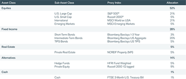
The portfolio is hypothetical and used for illustrative purposes only.

Principal Component Analysis

Just how diversified is this example portfolio based on a typical pension fund allocation? From a purely qualitative perspective, it appears to be a sensible allocation. It is diversified across asset classes, geographies, market caps, maturities and even includes a healthy dose of alternatives. A more rigorous inspection, however, reveals a very different reality. To assist in a more in-depth inspection, we have employed a quantitative technique known as Principal Component Analysis (PCA). PCA dissects large blocks of data into a more compact set of independent blocks. It divides the data into an ordered (by contribution to variance) set of independent views to provide an objective understanding of the number of contributing sources of variance and their relative importance.

Exhibit 2 presents the results of this analysis. As one can see, a U.S. pension fund based on this typical allocation would be surprisingly undiversified. Approximately 80% of the portfolio variance was caused by a single risk factor. The first two factors explained 90% of the portfolio risk.

Exhibit 2: Principal Component Analysis

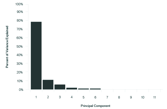
Analysis of the hypothetical portfolio proxied by indices representing the subasset classes depicted in Exhibit 1 is for the period 6/30/98 through 6/30/18. The analysis above is based on a hypothetical portfolio and used for illustrative purposes only.

This PCA analysis in Exhibit 2 provides two key insights. First, this portfolio is diversified in name only. From an objective standpoint, there is really only one significant source of risk. While PCA analysis does not provide for a direct identification (name) of the underlying source of variance, we infer that in this case, the underlying source of portfolio risk is equity exposure and the other securities in the portfolio are, broadly speaking, subject to the same underlying pressures. For example, the HFRI Fund Weighted Index has typically been highly correlated with the broad U.S. equity markets despite the addition of a wide variety of strategies and asset classes.

Second, this PCA analysis reveals that there has been a significant failure to define and access a broadly diversified set of independent risk factor exposures, i.e., risk premia.

Metaphorically speaking, this is akin to mismanaging an insurance company’s portfolio of policies. Consider two cases. First, imagine a collection of 1,000 fire insurance policies issued to 1,000 separate, unrelated homeowners. The insurance company is receiving a premium from each of the insured households for accepting the risk that their house might burn down. Assume that each house is completely isolated in the middle of a large concrete expanse. Further assume that there is a 0.001 (1/1,000) probability in any year of someone from any given home accidentally triggering a fire that destroys it. The portfolio of risk premia that the insurance company has assembled in this first case would be well structured due to its high degree of diversification. Provided that there are no other overlapping factors, the probability (p) of any house burning down in any given year would be 0.001, and the probability of it not burning down in any given year due to its assumed independence is (1 – p) = (1 – 0.001) = 0.999; essentially, no one house fire can trigger a fire in any other given home.

In the second case, this same group of families and their associated insurance policies have been transferred to a very compact neighborhood consisting of 1,000 quaint, wooden Victorian homes. In this situation, one miscue while preparing a BLT sandwich could not only cause a single home to burn down, it could also cause the entire compact wooden neighborhood to go up in flames as well. In this situation, the probability of not having to pay out on any single house has now decreased dramatically and is, in fact, due to the high degree of correlation associated with such a compact neighborhood, equal to the probability that none of them has a fire that year. The probability of not having a payout on any single home is calculated as: (1 – p)ⁿ = (1 – 0.001)¹⁰⁰⁰ = 0.37. In short, there is approximately a 63% (i.e., 1 – 0.37) chance the insurance company will have to pay out on any single home. Due to the assumed high degree of dependence, that figure is now equal to the probability of having to pay out on every single home in the neighborhood! Goodbye, insurance company.

Basic Portfolio Math

In the case of an investment portfolio, the math is more complicated, but the results can be just as striking.

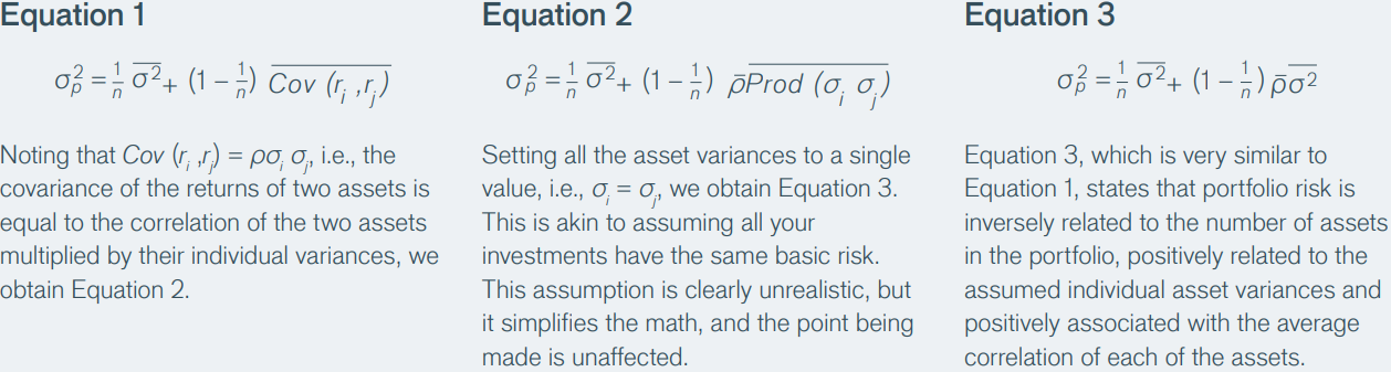
Equation 1, presented below, is a standard representation of the mathematical reality faced by investors. Reading from left to right, it states that portfolio risk, or variance, is inversely related to the number of assets in the portfolio, positively related to the average riskiness of the individual assets and positively related to their degree of statistical dependence.

Click an equation below to enlarge.

Impact of Correlation

Armed with Equation 3 from above, we can now “plug and play,” and perform a thought experiment. The purpose of this thought experiment is to develop a deeper visceral understanding of just how powerful an ally low-correlated risk premia can be to an investor.

Exhibit 3, presented below, summarizes the thought experiment. Assume we have created six portfolios. Each portfolio consists of a collection of individual assets, with each asset having an expected annualized return of 10% and an expected annualized volatility of 10%. The first five portfolios contain assets that have an assumed correlation (within their respective portfolios) of 0.5. The sixth portfolio contains assets with an assumed correlation of 0.0. The number of assets in each portfolio is shown below.

Exhibit 3: Impact of Correlation

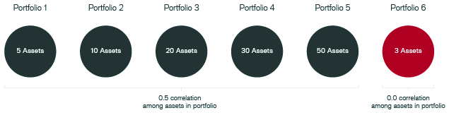
These portfolios are hypothetical and used for illustrative purposes only.

The question is, Which portfolio is better? To answer this question, we make use of Equation 3 to produce the output in Exhibit 4. The curved line shows how the annualized volatility decreases as we include an ever-larger number of assets in a given portfolio. The curve is derived by inserting the assumed values for correlation, volatility and the number of assets.

Exhibit 4: The Relationship Between Volatility, Correlation and the Number of Assets

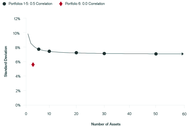
These portfolios are hypothetical and used for illustrative purposes only.

From the curved line in Exhibit 4, we see that as the number of assets in the portfolio increases, the volatility decreases. It decreases fairly rapidly for the first 10 assets, but after that it doesn’t really reduce the volatility significantly. In fact, an infinite number of 0.5-correlated assets won’t cause the volatility of the overall portfolio to drop below approximately 7.1%.

In contrast, the volatility of the three-asset Portfolio 6 is only 5.77%, which is almost 20% lower than a portfolio consisting of an infinite number of 0.5-correlated assets. The ability to invest in lowcorrelated assets sourced from statistically independent risk premia can provide a significant theoretical advantage when building a portfolio.

This is not the end of the story, however. The three-asset portfolio is not only less volatile, but it provides a higher geometric mean return as well, also known as growth rate of wealth, as shown in Exhibit 5.

Exhibit 5: Geometric Mean Return

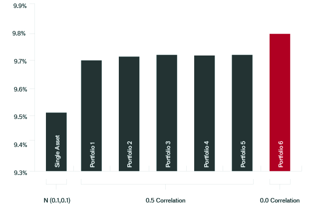
The rates of return are hypothetical and do not represent the returns of any particular investment.

This occurs because, as we see from Equation 4 below, there is a direct analytical linkage between the growth rate of wealth r, the arithmetic mean return x– and volatility σ².

The connection is that the growth rate of wealth is approximately equal to the arithmetic mean return minus a volatility correction. All else being equal, the lower the volatility of a portfolio, the higher the growth rate of wealth over time. As a result, the ability to invest in low-correlated assets, such as those based on low-correlated risk premia, may not only assist in controlling risk but also may contribute to higher returns.

The Moral of the Story

First, most portfolios invested in multiple asset classes may be diversified in name only, which may result in risk exposure concentrated in one or two risk factors. Second, diversification based on statistically independent risks can be effective for both reducing risk and enhancing returns. Thus, building a portfolio of low-correlated, well-defined, independent risk premia can potentially enhance performance outcomes to an extent that goes beyond many investors’ intuitive expectations.

---

¹ For a more detailed explanation of risk premia, that is, compensation for assumed risk, please see our paper titled “Introduction to Risk Premia Investing: Definitions and Examples.”
² Merthaler, Karl and Zhang, Helen. “Public Pension Funds: Asset Allocation Strategies,” JPMorgan Investment Analytics and Consulting, June 2010.